In this tutorial, we’ll explore using the VLOOKUP function in Microsoft Excel, one of the most powerful functions that Excel users may find under the different versions of MS Office Excel along with other useful functions that pivot tables. What VLOOKUP —Vertical Look Up—does is look for a value in the first column and also gives a value from another column. It is best if you type in the data for A1 to C10 from the sample table for this tutorial located below.
The formula for VLOOKUP is = VLOOKUP(X target, starting cell:X ending cell). For the example below for instance, it will be = VLOOKUP(1,A2:C10,2). This means we are looking for the closest instance less than or equal to 1. To start, put the formula in the formula bar (fx).

When you press Enter, it will go with the closest number to 1 in the A column—which is 0.946—and return with a number from the same row—in this case 2.17.

If we use the same formula, but add FALSE–= VLOOKUP(1,A2:C10,2, FALSE)—Excel will look for exact numbers. In the case below it turns up with #N/A meaning no such instance can be found within the data given.

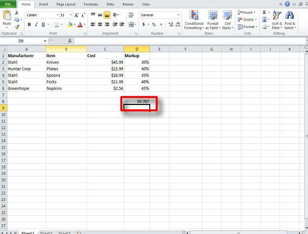
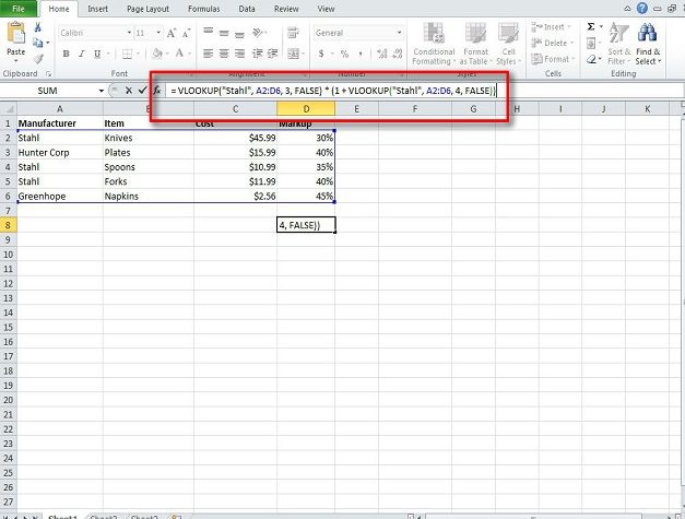
Finally, we will an example of a more specific VLOOKUP function in a business setup. Please type the below table into Excel.

Here, we will calculate the retail price knives. Type the following formula into the formula bar: = VLOOKUP(“Stahl”, A2:D6, 3, FALSE) * (1 + VLOOKUP(“Stahl”, A2:D6, 4, FALSE)).
The result will be 59.787. A number of operations can be done including subtracting a certain percent off of the listed price—use the same formula and after the * put (1 – 20%)—and so on.